AbstractPurpose:The aim of this study was to evaluate the performance of a proposed computer-aided detection (CAD) system in automated breast ultrasonography (ABUS).
Methods:Eighty-nine two-dimensional images (20 cysts, 42 benign lesions, and 27 malignant lesions) were obtained from 47 patients who underwent ABUS (ACUSON S2000). After boundary detection and removal, we detected mass candidates by using the proposed adjusted Otsu's threshold; the threshold was adaptive to the variations of pixel intensities in an image. Then, the detected candidates were segmented. Features of the segmented objects were extracted and used for training/testing in the classification. In our study, a support vector machine classifier was adopted. Eighteen features were used to determine whether the candidates were true lesions or not. A five-fold cross validation was repeated 20 times for the performance evaluation. The sensitivity and the false positive rate per image were calculated, and the classification accuracy was evaluated for each feature.
Results:In the classification step, the sensitivity of the proposed CAD system was 82.67% (SD, 0.02%). The false positive rate was 0.26 per image. In the detection/segmentation step, the sensitivities for benign and malignant mass detection were 90.47% (38/42) and 92.59% (25/27), respectively. In the five-fold cross-validation, the standard deviation of pixel intensities for the mass candidates was the most frequently selected feature, followed by the vertical position of the centroids. In the univariate analysis, each feature had 50% or higher accuracy.
Screening ultrasonography (US), as an adjunct to mammography, increases the sensitivity of the evaluation, particularly in the case of dense breasts [1-3]. However, hand-held US (HHUS) is operator dependent and time-consuming for whole breast evaluation. To overcome these problems, several automated breast US (ABUS) machines have been developed [4,5].
Several studies have shown that the ABUS is feasible [6-8]. ABUS can provide a high sensitivity similar to that of HHUS [9,10]. Kelly et al. [3,11] showed that the addition of ABUS to mammography improved cancer detection and made it possible to detect smaller cancer compared with mammography alone. However, there has been controversy about the sensitivity of ABUS. In some studies, ABUS exhibited a sensitivity that was as high as that of HHUS [9,10]. Other studies showed lower sensitivity than expected [12,13]. The high false-positive rate of ABUS is also problematic [9,10,12].
Furthermore, ABUS provides numerous images with a large field of view (FOV). The considerably large number of images provided by ABUS can lead to radiologist fatigue during interpretation. Subtle findings in a large FOV as well as the abovementioned fatigue can lead to a failure of lesion detection. More training or the application of a computer-aided detection (CAD) system may help to overcome these problems. The purpose of this study was to evaluate the performance of the proposed CAD system in ABUS.
The US images used in this study were provided by our hospital. The images were collected prospectively from October 1 to December 31, 2010. Informed consent was obtained from all the considered patients. This study protocol was reviewed and approved by the Institutional Review Board of our hospital. Ultrasonography was performed by two trained technologists by using ABUS (ACUSON S2000, Siemens Healthcare, Erlangen, Germany) with a largefootprint wide-frequency-bandwidth transducer (5-14 MHz; center frequency, 9 MHz). A volume of up to 15.4 cm├Ś16.8 cm├Ś6 cm was captured by the acquisition of a series of 320 high-resolution axial images at a slice thickness of 0.5 mm. All malignant lesions were pathologically diagnosed by biopsy or surgery. The benignity of the benign lesions considered in our study was pathologically determined by biopsy or indicated by a demonstration of stability for 2 years or longer [14].
The database consisted of the following three classes: a, cyst (n=20); b, benign lesion (n=42); and c, malignant lesion (n=27). Each class was composed of two-dimensional (2D) images. Images that were 707├Ś463 pixels in size were used with the center at the seed point, placed by the consensus of two radiologists with 4 years and 12 years of experience in breast imaging, respectively. There were 89 2D images taken from 47 patients. Some patients presented with multiple lesions. The number of lesions per patient varied from 1 to 8 (mean, 1.89 lesions/patient). To avoid redundancy, only one seed point was placed within a quadrant of a breast. The average size of the malignant or benign lesions was 25.61 mm (median size, 21 mm; size range, 5 to 81 mm) for malignant tumors, 11.56 mm (median size, 10.1 mm; size range, 5 to 26 mm) for benign lesions, and 8 mm (median size, 7.4 mm; size range, 4 to 14.4 mm) for cysts.
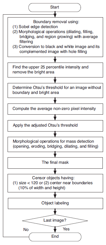
In general, the CAD system consists of data input, lesion detection with segmentation, and false positive reduction by classification. In the lesion detection process, we first removed the boundary area of an image, which is the border area having low pixel intensity outside of the breast in a given image. For the proposed CAD system, which was developed for research purposes only, boundary detection and removal based on edge detection and morphological operations including dilating, hole filling, bridging, region growing, and eroding as well as an average low-pass filtering were performed in the lesion detection process [15].
Once the boundaries were removed, areas with very bright intensities were also excluded. A bright area was determined by finding the top 25th percentile pixel intensity from the highest intensity values of the batch images. Then, the adjusted Otsu's threshold was applied in order to detect and segment the mass candidates.
Otsu's threshold is one of the most widely used pixel-intensity-based methods for lesion detection and segmentation [16]. However, the problem is that the detection and segmentation results obtained using Otsu's threshold are often unsatisfactory. For instance, Fig. 1A illustrates two Otsu's threshold values obtained for the mass candidates. For the Otsu's threshold represented by the left solid line, the pixel intensities for the mass candidates are located below the threshold, and the detection is assumed to be quite accurate. However, the true pixel intensities for the mass candidates are located between the solid and the dotted lines; thus, the abovementioned Otsu's threshold value fails to detect the lesions. Instead, the right dotted line represents the appropriate Otsu's threshold. In actual ABUS images, it was difficult for a CAD system to locate the true intensity values for the mass candidates since there were many factors affecting image intensities, including the anatomical variations of the patients and the scanner parameters. Fig. 1B illustrates a case where the intensity values of the mass candidates are not differentiated because of the smooth distribution of the intensity values.
As we observe in Fig. 1A and B, the effectiveness of Otsu's threshold is influenced by the original Otsu's threshold and the distribution of the intensity values. We analyzed the images whose boundaries and top 25th percentile bright areas were removed. For the detection and segmentation of mass candidates, we proposed an adjusted Otsu's threshold. The proposed adjusted Otsu's threshold, Adj.Otsu's Th, is as follows:
where Otsu's Th denotes the original Otsu's threshold (which implies a pixel intensity level that maximizes the between-class variance) and ╬▒ represents a model parameter (a slope term in a linear model for correcting the original Otsu's threshold by reflecting the anatomical variations of the patients and the scanner parameters). To model ╬▒, we manually found the lowest Otsu's threshold values that detected the mass candidates correctly while similarly sustaining the corresponding shapes. Then, ╬▒ was fit by using other variables such as the average non-zero pixel value for a masked image and the original Otsu's threshold because the adjusted Otsu's threshold was assumed to be related to the distribution of pixel intensities and the original Otsu's threshold. As a result, we observed that ╬▒ is proportional to the average non-zero pixel value and inversely proportional to the original Otsu's threshold as follows:
A global estimate for ╬▒ was found to be 0.003764 from 10 data samples; resulting inthe coefficient of determination, R2, as 99.6%. Fig. 1C shows the linear relation between ╬▒ and
in (2).
To achieve precise segmentation, several morphological operations, including opening, eroding, bridging, dilating, and hole filling, followed the detection using the proposed adjusted Otsu's threshold. Among the resulting objects, the ones that were very small were removed from the mass candidates (pixel area of less than 120, which is equal to approximately 3.5 mm├Ś3.5 mm). Likewise, objects located within 10% of the image width or height from the image boundaries were not considered masses. Finally, the segmented objects were labeled as either 0 or 1 depending on whether they belonged to the masses confirmed by the radiologists. Fig. 2 illustrates the described processes for the proposed CAD system.
After the detection, segmentation, and labeling of the mass candidates were completed, the features of the segmented objects were extracted and used for training and testing in the classification. To determine whether a mass candidate was a true lesion or not, we chose 18 extracted features from each segmented mass candidate (Table 1). We proposed two of these features for this study (features 17 and 18). These two features can be further described as follows:
Feature 17 (object boundary_mean) and feature 18 (object boundary_standard deviation) were added in the CAD system (Fig. 3). These features were based on the idea that the margin of a mass plays a role in the differentiation between benignity and malignancy. Feature 17 (object boundary_mean) is the mean pixel intensity of the object boundary and four of its neighboring pixels (in other words, the pixels on the left, right, top, and bottom of the pixel on the original boundary). Feature 18 is the standard deviation of the pixel intensity of these five pixels.
Elimination of the unwanted features and development of CAD with the most contributive features often improve the performance of a classifier. Irrelevant features only contribute to the generation of redundancy of the feature space, and thereby result in performance degradation in terms of accuracy in addition to increasing the number of computations. Sequential forward selection is one of the feature selection methods used in classification. In sequential forward selection, features are added one-by-one to the current feature set until the performance of the given model stops improving by the addition of a new feature.
Cross validation is a method for estimating accuracy in classification. k-fold cross validation splits data into k subgroups that are almost equal in size. Then, we build a classification model using k -1 subgroups (training data). Once a classification model is determined, the model is fit to the remaining subgroup data called a test set, and the accuracy for the test set is measured (Fig. 4) [17].
In the proposed CAD study, class 0 was defined as a set of mass candidates that were a portion of normal tissue (that is, true negative), and class 1 was defined as a set of mass candidates that were either benign masses or malignant masses or cysts (that is, true positive). The true masses that were not detected by CAD (false negative cases) were not included in any class. We obtained 1,095 data that belonged to either class 0 or class 1, which corresponded to the set of non-masses and that of masses, respectively. The number of correctly detected masses was 83 out of 89, and these masses were classified into class 1. The rest 1,012 (=1,095-83) datawere labeled as class 0. To prevent a biased estimate for the classification accuracy due to the difference in the data sizes, we randomly selected 83 data from class 0. Then, we merged the 83 data of class 1 with the randomly sampled 83 data of class 0 and applied five-fold cross validation. We repeated this process 20 times in order to measure the classification accuracy as shown in Fig. 4.
Some studies used a support vector machine (SVM) for the diagnosis of breast cancer using ultrasonography [18-21]. A linear SVM learns to distinguish between negative (normal tissue) and positive (mass) cases by constructing an optimal separating hyperplane. The optimal hyperplane leaves the largest fraction of the same class on the same side and maintains a maximal distance from either class. In this study, an SVM with a nonlinear classifier based on a radial basis function was used for each cross validation. First, we applied univariate classification with the SVM, which used each of the considered features. Then, we used all the 18 features for building the final SVM classifier. The library for SVM (LIBSVM) was utilized for the implementation of the SVM classification [22].
To measure the effectiveness of the proposed CAD system, we computed the sensitivity, false positive rate per image, and accuracy of each feature in the classification using five-fold cross validation that was repeated 20 times. Sensitivity is calculated by dividing the number of the objects which were correctly classified asmasses by the total number of true mass The term ŌĆ£false positive objectsŌĆØ refers to mass candidates that were not true masses but normal breast tissue. In the detection step, it was difficult to define a negative case since the negative case was referred to as the whole area of images in which no mass is detected. However, in the classification step, the number of samples including both positive labels and negative labels, which corresponded to masses and nonmasses, respectively, was known in the cross validation. We set both the number of masses and that of non-masses to 83. To determine the classification accuracy of the proposed CAD system, we first computed the sum of the number of correctly classified masses and that of correctly classified non-masses. Then, this result was divided by the sum of the number of sampled masses and the number of sampled non-masses, as in (3)
We also evaluated the possible causes of the false negative cases, that is, cases in which the proposed CAD system did not detect the true mass.
To measure the effectiveness of the proposed CAD system, we computed the sensitivity and the false positive rate of the classification by using a five-fold cross validation. We calculated the sensitivity to be 82.67%┬▒0.02% and the false positive rate to be 0.26 per image.
We also computed sensitivities for benign and malignant mass detection, which were 90.47% (38/42) and 92.59% (25/27), respectively, at the detection/segmentation step. All the cysts were detected at the detection/segmentation step. The lesion detected by the proposed CAD system is shown in Fig. 5.
There were two possible causes of failure in the detection of masses. Inaccurate segmentation was the first one. Some missed cases were segmented smaller than their true size and removed due to the small size (less than 120 pixels) or segmented unsuitably. The second possible cause was the inaccurate removal of mass candidates according to their location in the considered image. In some false negative cases, the true masses were removed during the removal of mass candidates within 10% of the image width or height from the image boundary (Fig. 6). The characteristics of the missed cases are given in Table 2.
The order of the detection power of each feature is given in Table 3. All the features had 50% or more accuracy of lesion detection when inserted in the proposed CAD system alone. The results of sequential forward feature selection during the 20 rounds of cross validation are presented in Table 4. The best accuracy was 89.80%; it was obtained when five features, namely features 2, 6, 7, 1, and 13, were used. The order of addition during forward feature selection is given in Table 5. In the five-fold cross validation, the standard deviation of the pixel intensities of the mass candidates were the most frequently selected feature followed by the vertical position of the centroid, the size of the bounding boxes, the convex area, the average intensity of the pixels, and the mean pixel intensity of the object boundary. All the benign lesions and cysts were assigned as Breast Imaging Reporting and Data System (BI-RADS) category 2. The BI-RADS categories of all considered and missed malignant lesions are listed in Table 6.
ABUS reduces many shortcomings of HHUS, such as operator dependency, and provides high-resolution three-dimensional (3D) images. However, the considerable number of images with a large FOV provided by ABUS can lead to a failure of lesion detection due to radiologist fatigue during interpretation and subtle findings in a large FOV. Several studies have suggested that a precise interpretation of ABUS requires substantial training and experience [4,12]. As with other CAD systems in other imaging modalities such as chest computed tomography, CT colonography, or mammography, CAD system for ABUS can improve the radiologistŌĆÖs performance in the detection of masses in ABUS.
The sensitivities and the false positive rates of the previous CAD systems in ABUS were 70% with 2.7 false positives per pass [23] and 64% with 1 false positive per image [24]. The proposed CAD had substantial sensitivity as compared to the previous methods. The sensitivity during detection and segmentation in the case of the proposed CAD system was 93%, and the cross validation estimated a sensitivity of 82.67%┬▒0.02% with 0.26 false positives per image. Because most of the cases missed by the proposed CAD system were not detected during the false positive reduction (such as censoring according to the location or removal of objects that were less than 120 pixels in size), modification of the level of false positive reduction is likely to improve the sensitivity of the proposed CAD system.
Four benign masses and two malignant masses were not detected. Except one malignant mass (size, 23 mm), the missed lesions were less than 8 mm in size (average, 5.88 mm; range, 5 to 7.4 mm).
We adopted the adjusted Otsu's threshold for segmentation and detection based on the pixel intensity. The pixel intensity was used in most of the previous CAD systems [4,25]. We found that the results of the proposed CAD system were similar to those of a previous CAD system using a blob detection algorithm [23]. First, there were numerous false positives, and most of them were small in size (less than 120 pixels in our study). Second, some of the mass candidates were segmented smaller than their true size.
According to the univariate analysis, all the features had 50% or more accuracy. Feature 2, which reflects the heterogeneity of the mass candidates, had the highest discriminatory power. It was selected every time during the 20 repetitions of the cross validation and had the highest accuracy when inserted alone. This implies that a true positive lesion is more heterogeneous than a false positive mass candidate. The standard deviation of the pixel intensity is a unique feature, because we cannot easily notice the inner heterogeneity of the mass candidates with our naked eye.
The y-coordinate of the center of the mass candidate was the second most commonly selected feature by sequential forward selection. The y-axis is the vertical axis of the given image. This result agrees with the common knowledge. As the breast on an oval-shaped chest wall was scanned by using a flat transducer (dimensions, 15.4 cm├Ś16.8 cm), the semicircular black background and the chest wall where breast lesions could not arise were covered in the inferior aspect of the scanned image. The far upper portion of the scanned image would also not include many masses; most of the breast masses would arise in the parenchymal tissue rather than in the fat layer.
The third and fourth most commonly selected features were feature 7 (convex area) and feature 4 (bounding box). Because a larger mass has a larger convex area and bounding box, the proposed CAD system seems to consider a larger mass candidate to be a true positive lesion.
The fifth most frequently selected features were feature 1 (mean) and feature 17 (object boundary_mean). Between feature 1 and feature 17, feature 17 seemed to have more discriminatory power. Although the accuracy of feature 17 in the univariate analysis was of the last order, the number of second-order selections after feature 2 during the sequential forward selection was larger for feature 17 than for feature 1. This result implies that the mass candidate with a lower mean pixel intensity of the object boundary had a tendency to be regarded as a true positive lesion. Feature 1, which is the average intensity of pixels in the mass candidate, shows that a true positive mass candidate is darker than a false positive mass candidate. These findings agree with the general knowledge that most of the masses in the glandular tissue are hypoechoic as compared to the echogenic glandular tissue. As Otsu's threshold already discriminates mass candidates from normal tissue according to the pixel intensity (the lower area was detected as mass candidates), the discriminatory power was not as high as expected.
The proposed CAD system has some limitations. First, the sample size in each class was not equal between classes and was small for training a clinically robust classifier. A sufficient number of reference standards are required to develop a more accurate and clinically useful CAD system. Further, the development of a CAD system with more training data can improve the performance of the CAD system. Second, there was a difference in the data storage techniques between malignant lesions and the other classes. Only post-processing data, some of whose information was deleted, were stored for certain cases in the malignant class. Finally, the adjustment of censoring according to the location from the image boundary and the size of the mass candidates might be further calibrated to improve the classification performance.
In order to reduce the radiologistsŌĆÖ burden, we proposed a CAD system for the most recently developed and more widely used ABUS. The proposed CAD system is based on detection and segmentation with a simple adjusted Otsu's threshold and classification with a nonlinear SVM classifier. The proposed CAD has accuracy substantially higher than the accuracy of the previously reported methods. The sensitivity during detection and segmentation in the case of the proposed CAD system is 93%, and the cross validation estimates the sensitivity to be 82.67%┬▒0.02%.
AcknowledgementsThis research was supported by Basic Science Research Program through the National Research Foundation of Korea (NRF) funded by the Ministry of Education, Science and Technology (No. 2011- 0014033).
References1. Kolb TM, Lichy J, Newhouse JH. Occult cancer in women with dense breasts: detection with screening US. Diagnostic yield and tumor characteristics. Radiology 1998;207:191ŌĆō199.
2. Berg WA, Blume JD, Cormack JB, Mendelson EB, Lehrer D, Bohm-Velez M, et al. Combined screening with ultrasound and mammography vs mammography alone in women at elevated risk of breast cancer. JAMA 2008;299:2151ŌĆō2163.
3. Kelly KM, Dean J, Comulada WS, Lee SJ. Breast cancer detection using automated whole breast ultrasound and mammography in radiographically dense breasts. Eur Radiol 2010;20:734ŌĆō742.
4. Ikedo Y, Fukuoka D, Hara T, Fujita H, Takada E, Endo T, et al. Development of a fully automatic scheme for detection of masses in whole breast ultrasound images. Med Phys 2007;34:4378ŌĆō4388.
5. Youk JH, Kim EK. Supplementary screening sonography in mammographically dense breast: pros and cons. Korean J Radiol 2010;11:589ŌĆō593.
6. Destounis S, Young W, Murphy P, Somerville P, Seifert P, Zuley M. Initial experience of automated breast ultrasound screening trial in the setting of a community based private practice [abstract]. RSNA 2006;2006 Nov 26-Dec 1; Chicago, IL, USA.
7. Destounis S, Young W, Hanson S, Somerville P, Murphy P, Zuley M. Automated breast ultrasound: a pilot study [abstract]. RSNA 2005;2005 Nov 27-Dec 2; Chicago, IL, USA.
8. Wenkel E, Heckmann M, Heinrich M, Schwab S, Uder M, Schulz-Wendtland R, et al. Automated breast ultrasound: lesion detection and BI-RADSŌäó classification-a pilot study. Fortschr R├Čntgenstr 2008;180:804ŌĆō808.
9. Wojcinski S, Farrokh A, Hille U, Wiskirchen J, Gyapong S, Soliman AA, et al. The Automated Breast Volume Scanner (ABVS): initial experiences in lesion detection compared with conventional handheld B-mode ultrasound. A pilot study of 50 cases. Int J Womens Health 2011;3:337ŌĆō346.
10. Lin X, Wang J, Han F, Fu J, Li A. Analysis of eighty-one cases with breast lesions using automated breast volume scanner and comparison with handheld ultrasound. Eur J Radiol 2012;81:873ŌĆō878.
11. Kelly KM, Dean J, Lee SJ, Comulada WS. Breast cancer detection: radiologists' performance using mammography with and without automated whole-breast ultrasound. Eur Radiol 2010;20:2557ŌĆō2564.
12. Chang JM, Moon WK, Cho N, Park JS, Kim SJ. Breast cancers initially detected by hand-held ultrasound: detection performance of radiologists using automated breast ultrasound data. Acta Radiol 2011;52:8ŌĆō14.
13. Chang JM, Moon WK, Cho N, Park JS, Kim SJ. Radiologists' performance in the detection of benign and malignant masses with 3D automated breast ultrasound (ABUS). Eur J Radiol 2011;78:99ŌĆō103.
14. Graf O, Helbich TH, Hopf G, Graf C, Sickles EA. Probably benign breast masses at US: is follow-up an acceptable alternative to biopsy? Radiology 2007;244:87ŌĆō93.
15. Gonzalez RC, Woods RE, Eddins SL. Digital image processing using MATLAB. 2nd ed. Natick, MA: Gatesmark Publishing, 2009.
16. Ostu N. A threshold selection method from gray-level histogram. IEEE Trans Syst Man Cybern 1979;9:62ŌĆō66.
17. Hastie T, Tibshirani R, Friedman J. The elements of statistical learning; data mining, inference, and prediction. 1st ed. New York: Springer-Verlag, 2001.
18. Chang RF, Wu WJ, Moon WK, Chou YH, Chen DR. Support vector machines for diagnosis of breast tumors on US images. Acad Radiol 2003;10:189ŌĆō197.
19. Huang YL, Chen DR. Support vector machines in sonography: application to decision making in the diagnosis of breast cancer. Clin Imaging 2005;29:179ŌĆō184.
20. Chang RF, Wu WJ, Moon WK, Chen DR. Improvement in breast tumor discrimination by support vector machines and speckleemphasis texture analysis. Ultrasound Med Biol 2003;29:679ŌĆō686.
21. Chen ST, Hsiao YH, Huang YL, Kuo SJ, Tseng HS, Wu HK, et al. Comparative analysis of logistic regression, support vector machine and artificial neural network for the differential diagnosis of benign and malignant solid breast tumors by the use of three-dimensional power Doppler imaging. Korean J Radiol 2009;10:464ŌĆō471.
22. Chang CC, Lin CJ. LIBSVM: a library for support vector machines. ACM Trans Intell Syst Technol 2011;2:27.
23. Moon WK, Shen YW, Bae MS, Huang CS, Chen JH, Chang RF. Computer-aided tumor detection based on multi-scale blob detection algorithm in automated breast ultrasound images. IEEE Trans Med Imaging 2013;32:1191ŌĆō1200.
Distribution of pixel intensities and Otsu's thresholds.A. Otsu's threshold values are represented by a solid line and a dotted line. If the pixel intensities of a mass candidate are located below the solid line, the mass candidate can be detected by both the lines. However, the mass candidates whose pixel intensities are located between the solid and the dotted line cannot be detected by the computer-aided detection (CAD) system with the Otsu's threshold value represented by the dotted line (x-axis, pixel intensity; y-axis, number of pixels). B. The intensity values of mass candidates are not differentiated because of the smooth distribution of the intensity values (x-axis, pixel intensity; y-axis, number of pixels). C. This graph shows the relation between ╬▒ and the average non-zero pixel value divided by the original Otsu's threshold (x-axis, average non-zero pixel value for a masked image divided by the original Otsu's threshold; y-axis, the lowest Otsu's threshold values obtained from a manual adjustment to detect the mass candidates correctly).
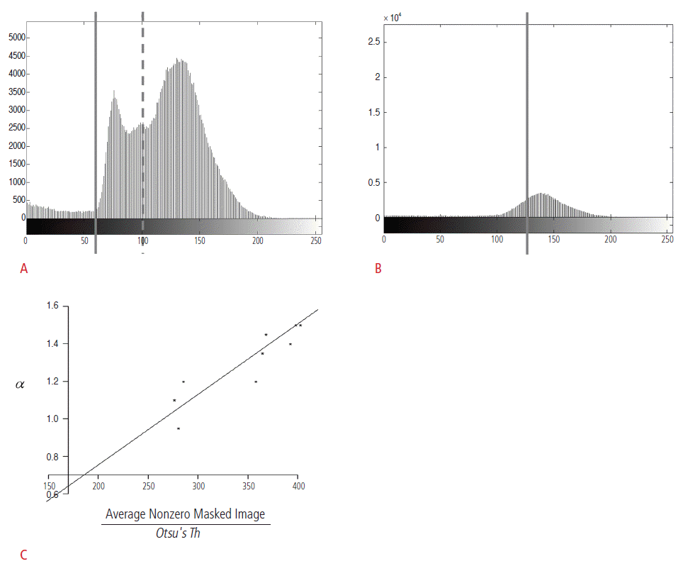 Fig.┬Ā1.The concepts of feature 17 (object boundary_mean) and feature 18 (object boundary_standard deviation).One box in the illustration denotes one pixel. Black and gray boxes represent the boundary of an object. The gray box denotes the pixel of interest on the boundary. The mean pixel intensity of the boundary (feature 17) is the mean pixel intensity of the gray box and that of the boxes with letters A (top), B (left), C (bottom), and D (right). The standard deviation of the pixel intensity of the boundary (feature 18) is the standard deviation of the abovementioned five pixels.
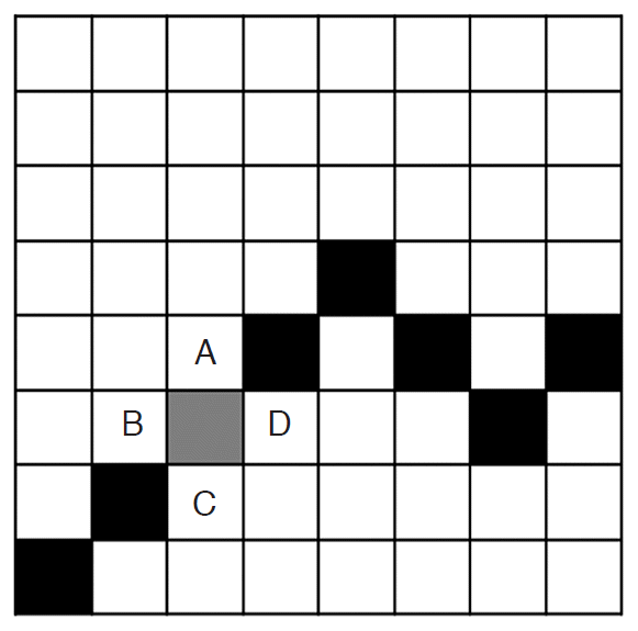 Fig.┬Ā3.The example of k-fold cross validation.The dataset is divided into k subsets. One set is used for testing (black boxes), and the remaining k- 1 subsets (empty boxes) are used for training. Then, the entire dataset is again divided into k subsets, which are different from the abovementioned k subsets. Then, training and testing are carried out. These steps are repeated 20 times.
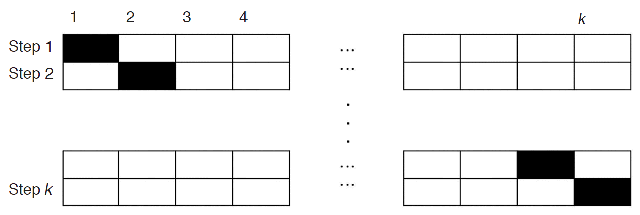 Fig.┬Ā4.True positive case in a 46-year-old female with a pathologically proven fibroadenoma in her right breast.A. The original automated breast ultrasonogram shows a 1.84-cm circumscribed hypoechoic nodule (fibroadenoma). B. The final mask after the adjusted Otsu's threshold and mor-phological operations shows mass candidates in white. C. The gray-scaled frame with the final mask reveals the true positive object (circle) and the false positives (some of which will be removed from the final mask after support vector machine classification).
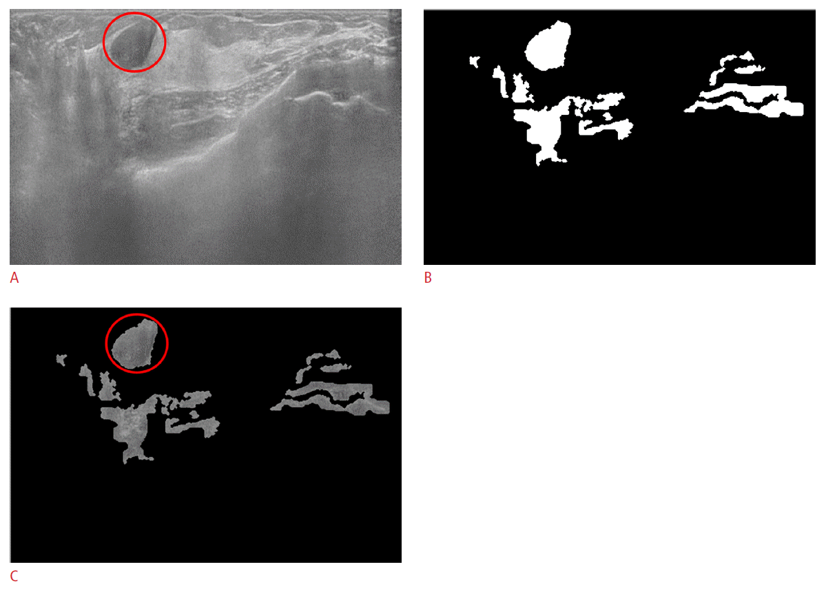 Fig.┬Ā5.False negative case in a 53-year-old female with an isoechoic nodule in her left breast, which has been stable for 2 years.A. The original automated breast ultrasonogram shows a 6-mm isoechoic nodule (circle) in the left subareolar area. B. The true nodule is detected before being censored by size and location. C. The final mask after censoring by size and location demonstrates only false positive mass candidates. D. The gray-scaled frame after applying the final mask shows only false positive mass candidates.
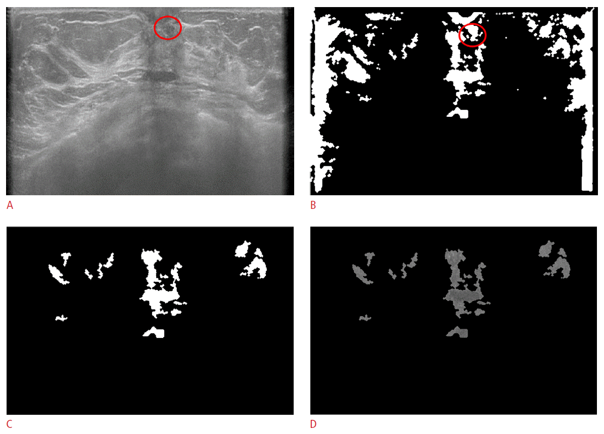 Fig.┬Ā6.Table┬Ā1.Overview of features used as classifiers of the computer-aided detection system Table┬Ā2.Characteristics of missed cases Table┬Ā3.Order of detection power of 18 features obtained by univariate analysis Table┬Ā4.Results of sequential forward feature selection Table┬Ā5.Order of addition during forward feature selection |


 Print
Print facebook
 twitter
 Linkedin
 google+
 Download Citation
 PDF Links
 PubReader
 ePub Link
 Full text via DOI
 Full text via PMC


