High-spatial-resolution, instantaneous passive cavitation imaging with temporal resolution in histotripsy: a simulation study

Article information

Ultrasonography. 2022;41(3):566-577

Publication date (electronic) : 2022 February 22

doi : https://doi.org/10.14366/usg.21153

Mok Kun Jeong ¹

, Min Joo Choi ²

, Sung Jae Kwon^,³

¹Department of Electronic Engineering, Daejin University, Pocheon, Korea

²Department of Medicine, Jeju National University, Jeju, Korea

³Division of IT Convergence Engineering, Daejin University, Pocheon, Korea

Correspondence to: Sung Jae Kwon, PhD, Division of IT Convergence Engineering, Daejin University, 1007 Hoguk-ro, Pocheon 11159, Korea Tel. +82-31-539-1923 Fax. +82-31-539-1890 E-mail: sjkwon@daejin.ac.kr

Received 2021 July 27; Revised 2022 February 21; Accepted 2022 February 22.

Abstract

Purpose

In histotripsy, a shock wave is transmitted, and the resulting inertial bubble cavitation that disrupts tissue is used for treatment. Therefore, it is necessary to detect when cavitation occurs and track the position of cavitation occurrence using a new passive cavitation (PC) imaging method.

Methods

An integrated PC image, which is constructed by collecting the focused signals at all times, does not provide information on when cavitation occurs and has poor spatial resolution. To solve this problem, we constructed instantaneous PC images by applying delay and sum beamforming at instantaneous time instants. By calculating instantaneous PC images at all data acquisition times, the proposed method can detect cavitation when it occurs by using the property that when signals from the cavitation are focused, their amplitude becomes large, and it can obtain a high-resolution PC image by masking out side lobes in the vicinity of cavitation.

Results

Ultrasound image simulation confirmed that the proposed method has higher resolution than conventional integrated PC imaging and showed that it can determine the position and time of cavitation occurrence as well as the signal strength.

Conclusion

Since the proposed novel PC imaging method can detect each cavitation separately when the incidence of cavitations is low, it can be used to monitor the treatment process of shock wave therapy and histotripsy, in which cavitation is an important mechanism of treatment.

Keywords: Beamforming; Passive cavitation imaging; Strength of cavitation

Introduction

Short-pulse, high-amplitude ultrasonic therapy such as lithotripsy or histotripsy is an effective noninvasive therapeutic approach that relies on mechanical effects generated by collapsing bubbles. Extracorporeal shock wave lithotripsy is an example of a noninvasive technique used to treat urinary lithiasis; this method fragments stones through cavitation-induced erosion caused by the violent collapse of bubbles near the surface of the stone [1-4]. The cavitation generated when a bubble collapses mechanically disrupts soft tissue, and this effect is used to treat tumors in soft tissue. Using focused ultrasound delivered from outside the body, histotripsy produces tissue fractionation through cavitation, rendering the target into acellular debris [5-10]. There is an increasing need for improving the safety and efficacy of the treatment process, as well as reducing side effects, by continuously monitoring microbubbles and providing feedback [11-14].

In ultrasound imaging, microbubble monitoring can be divided into active or passive acoustic monitoring. An active bubble image is obtained in the same manner as a conventional ultrasound B-mode imaging system [15,16]. An ultrasound wave for imaging is transmitted, and echoes from bubbles are imaged due to the difference in acoustic impedance between soft tissue and bubbles [17]. Since the transmission of an ultrasound wave may affect the activity of bubbles, a variety of transmitting sequences are applied to avoid damaging the surrounding tissue by cavitation until the bubbles arrive at the target for treatment [14].

Passive cavitation (PC) imaging maps the acoustic emissions from the cavitation bubbles without separately transmitting ultrasound waves for imaging [18-23]. In cavitation-cloud histotripsy or extracorporeal shock wave lithotripsy, a transmitted shock wave generates inertial cavitation in a medium after transmission [3,24-26]. Accordingly, there is a need to image and both temporally and spatially resolve cavitation bubbles over a long period with passively received radiofrequency (RF) data.

In dynamic receive beamforming, a focusing time delay is applied to the signals of all receive channels to maximize the amplitude of a signal coming from an imaging point to be focused. If there is a cavitation at the focused imaging point, it appears as a main lobe in the ultrasound field pattern, so a large signal appears. If the cavitation signal from outside the imaging point is not completely removed during the focusing process, it appears as a side lobe at the imaging point [27,28]. In general, the side lobe spreads widely over the image area, thus reducing the image contrast. Since PC imaging does not transmit an ultrasound wave, but only receives acoustic emissions from cavitation, the cavitation occurrence time is not available, and thus accurate receive focusing cannot be accomplished.

Therefore, conventional PC images are produced by integrating the energy of cavitation generated over the entire time interval during which cavitation occurs after only receive focusing is applied to the passively received data. Therefore, those images have no temporal resolution, and the contrast is poor due to side lobes generated during the receive focusing process. In particular, when a strong cavitation occurs, the side lobe signals that appear in the receive focusing process mask the signal from a weak cavitation with the result that the latter cannot be identified. Several research groups achieved temporal resolution by integrating signals within a short window, rather than over the entire time interval, and sliding the window [14,29]. Since they used the integration processing itself in receive focusing, the effect of side lobes could not be eliminated. To suppress side lobes, the minimum variance beamforming method has been widely used as a signal processing technique [30,31]. This method features increased ultrasound image quality, but it cannot completely remove the long tail streak and side lobe of a cavitation image due to the integration processing.

This paper proposes a PC imaging method that has temporal resolution by applying delay and sum beamforming at the specified time instants, as well as spatial resolution by masking out side lobes, using several hundred microseconds of passively received RF data in histotripsy. Since a cavitation signal can be assumed to be a point-like source, it will appear as a bright point in a PC image when the signal is properly focused on receive. In this method, a PC image is constructed at regularly spaced time instants and the maximum image pixel value is found. By repeating this process over the entire data acquisition time, a sequence of maximum pixel values is obtained, in which a local maximum indicates the occurrence of a cavitation. A computer simulation shows that when the frequency of cavitation occurrence is low, the method proposed herein can detect individual cavitations that do not overlap in time and space with high temporal and spatial resolution. The theoretical formulation of focusing in instantaneous PC imaging is described in the Materials and Methods section, and a numerical simulation of cavitation bubble collapse is presented in the Results section.

Materials and Methods

In conventional ultrasound B-mode imaging, the time delay for dynamic receive focusing can be computed since the receive process is synchronized with the transmit process. However, the dynamic receive focusing used in conventional ultrasound B-mode imaging cannot be used without modifications since PC imaging focuses only on receive using continuously received data. In this section, the authors propose a method to create a new PC image with time resolution by applying delay and sum receive focusing to passively received RF data over a long period of several hundred microseconds.

Instantaneous PC Imaging

Fig. 1 is a conceptual diagram of implementing PC imaging using acoustic signals generated in a medium at a certain time t₀. Here, x and z denote the lateral and axial direction, respectively. The acoustic signal generated at point P₁ is first received at time t_arrival by the ultrasound probe element nearest to P₁. Fig. 1B shows the RF data sampled and stored in the receive array by the acoustic signal starting at point P₁ at time t₀. Since signals sequentially arrive after time t_arrival at the receive array located at a farther distance from the signal generation position, they take an arc-shaped arrival time distribution in the RF data plane.

Fig. 1.

The medium, image, and radiofrequency (RF) data planes.

A. Acoustic emission that occurred at point P₁ in the medium plane at t₀ is propagated to the receiving array. B. The RF data are passively received by the linear array ultrasound probe and stored in memory. The arrival time of signals from point P₁ in the medium plane (time versus channel) takes the form of a curve. C. The arrival time curve of signals from point P₁ is the same as that of receive focusing curve P₁’. P₁ is assumed to have occurred at t₀. The RF data from point P₁ coincide with receive focusing curve P₁’. D. The RF data focused using receive focusing curve P₁’ are mapped to imaging point P₁. Since there are no RF data available in receive focusing curve P₂’, side lobes appear at P₂ since parts of P₁’ and P₂’ overlap.

Several acoustic signals generated simultaneously at time t₀ in a medium to be imaged are received within a certain time range after t₀ depending on the propagation distance. Since the shape of the channel-arrival time curve depends on the location or occurrence time, it is possible to find the location of the sound source in the medium from the shape and time location of the arrival time curve.

We compute the receive focusing time delay for the signal generated from a point P₁ in the medium at t₀. The time it takes the signal emitted from P₁ to arrive at each receive channel is computed as follows [30].

(1) τn(x,z)=(x-xn)2+z2c

x_n is the position of the nth receive element, and c is the sound velocity. Therefore, the signal arrives at each receive channel at time t₀+τ_n(x,z). Fig. 1C shows the arrival time, which differs for every imaging point. Fig. 1C is obtained by imposing the time delay for focusing the signal generated at P₁ at time t₀ in the RF data plane. Therefore, if all the data for the imaging point P₁ in Fig. 1C are added together in the RF data plane of Fig. 1B, the receive focusing for P₁ is accomplished. Since all the RF signals from the medium plane need to be added, the signal focused at the imaging point can be computed as follows [32]:

(2) s(x,z,t)t=t0=∑n=1Nrn(t+τn(x,z))

Here, r_n is the signal in the nth receive channel. Fig. 1C presents the arrival time curve of P₂' (dashed line). If a signal is not generated at point P₂ in the medium, no signal should appear at point P₂ of the image. However, when curve P₂' (dashed line) and curve P₁' (solid line) of the receive focusing intersect, and the signals from P₁ at the intersection are added together during the focusing process of imaging point P₂, a side lobe or clutter is created at P₂.

The instantaneous PC image observed at time t₀ is obtained by demodulating the focused RF signal given in Eq. (2), and is expressed as follows:

(3) Instantaneous PCI(x,z,t)t=t0=|s(x,z,t)t=t0|

where |·| stands for taking the absolute value, or performing demodulation. The instantaneous PC image obtained using Eq. (3) at time t₀ shows the spatial distribution of all ultrasonic signal generators at time t₀ in the medium plane of depth from z=0 to z=z_end. Cavitations that occur at other time instants are computed in the same way, by moving the time instant t₀ in the RF data plane.

Integrated PC Imaging

In conventional integrated PC imaging, a single image is obtained by applying the focusing delay to the entire series of time data and then integrating them over time. Therefore, the image has spatial resolution but not temporal resolution. The integrated PC image is obtained by accumulating Eq. (3) over time [33-35].

(4) Integrated PCI=∑t=0T|s(x,z,t)|2

Here, T denotes the time interval over which to acquire the data.

Results

A simulation study was performed to investigate the characteristics of the temporal and spatial resolution of instantaneous PC images. First, cavitation by a single bubble was considered, and based on this, computer simulations were performed on multiple cavitation events, including five bubbles with different rupture locations, times, and strengths.

Acoustic Emission and Passive Detection

The acoustic signal p(t) emitted as a result of cavitation is assumed to be a point source at the location of cavitation occurrence [35,36]. As shown in Eq. (5), p(t) is modeled as a short-time pulse with a Gaussian function shape (Fig. 2A).

Fig. 2.

Acoustic signal waveform and receive channel radiofrequency (RF) data.

A. The acoustic signal waveform p(t) due to bubble collapse is modeled as a short-time pulse in the form of a Gaussian function. B. The RF data for acoustic emission p(t) of a single bubble collapsing at z=30 mm passively detected by a 64-channel receiving system with a linear array ultrasound probe shows a curve shape in the time-channel representation. Note that the dotted line is the signal arrival time t_arrival and that the bubble collapse time is calculated by t₀=t_arrival-z/c.

(5) p(t)=exp(-ω02·t2/σ2)·cos(ω0t)

where the center frequency f₀= ω₀/2π and the pulse width parameter σ were set to 5 MHz and 2.5π, respectively. Passively received RF data were simulated by adding Gaussian noise to Eq. (5) so that the signal-to-noise ratio was 25 dB [37].

The ultrasonic signal emitted from cavitation was passively received. We used a 128-element linear ultrasound probe, but every other element was used for data acquisition. The effective pitch of the ultrasound probe elements was increased to 0.6 mm. Although the number of the receive channels was 64, the aperture width was increased, leading to improved resolution at the expense of generating grating lobes. The RF data were generated by sampling at a frequency of 40 MHz. All the simulations were performed on a PC using MATLAB (The MathWorks, Natick, MA, USA).

Single Cavitation

The single cavitation bubble considered in the simulation was positioned at a depth z=30 mm from the ultrasound probe. The propagation speed of sound was assumed to be 1,480 m/s.

Fig. 2B shows the RF data acquired in the 64 receive channels of the ultrasound probe in the time-channel area due to a cavitation that occurred at a depth of z=30 mm. If the cavitation occurrence time is t₀, then the time at which the emitted acoustic signal first arrives at the nearest receive element is t_arrival=t 0+z/c. This is the time indicated by the dashed line in Fig. 2B. Assuming that t₀=0 s and that the ultrasound probe element is located at the depth z=0 mm, it follows that t_arrival=20.27 μs.

Unlike the focusing process of a conventional medical ultrasound imaging system that uses transmit and receive focusing, in PC imaging the signal is generated from a point source. Therefore, if the focused imaging point coincides with the position of the point source, the effect is that the transmission focusing has already been carried out. Therefore, the imaging point where cavitation occurs has high resolution in the image since the focusing is performed effectively in both transmit and receive even though only receive focusing is done.

Using Eqs. (2) and (3), the instantaneous PC image from RF data (Fig. 2B) was constructed by applying time gating from the time instant at which the cavitation occurred (i.e., t=t₀), as shown in Fig. 3B. The produced image had a size of 10 mm×10 mm over a depth range of 25 mm to 35 mm around the depth z=30 mm at which the cavitation occurred. The resolution of the cavitation image depends on the performance of the focusing system and corresponds to its point-spread function (PSF). Therefore, the cavitation appears as the main lobe in the PSF of the imaging system, and other artifacts appear as side lobes. The instantaneous PC image obtained at the instant of cavitation occurrence has a high spatial resolution since the main lobe appears in a small area due to the beneficial effect of the transmit and receive focusing, and the side lobe artifacts around the main lobe are significantly reduced. However, in the integrated PC image (Fig. 3A), the main lobe is elongated along the axial axis, and large side lobes appear over a wide area. Fig. 3C shows a circular mask used to segment the cavitation. Fig. 3D shows a high-spatial-resolution cavitation image with the side lobe masked out. In practice, we cannot find the cavitation occurrence time from actual experimental data. To overcome this problem, we tracked the temporal variation of an instantaneous PC image.

Fig. 3.

Comparison of integrated and instantaneous passive cavitation (PC) images of a single cavitation.

A. Integrated PC image shows high side lobe levels. B. Instantaneous PC image constructed at t=t₀ shows high spatial resolution. C. A circular mask is placed where cavitation was detected. D. Integrated PC image with circular mask shows high-spatial resolution cavitation image with side lobe masked out. The images were normalized to the maximum value of each image to make its maximum brightness the same.

In instantaneous PC imaging, an image was constructed using the RF data present at the specific time instant. By moving the time instant on the time axis in the RF data plane, we can construct a number of instantaneous PC images having temporal resolution. Fig. 4 shows instantaneous PC images constructed at time intervals of 1 μs before and after the cavitation occurrence time t=t₀. In the temporally continuous PC images, as the time instant moves away from t=t₀, the position of the main lobe moves away from the position of cavitation, as its height decreases and shape changes. The area in which the side lobes are distributed also increases. When computing the instantaneous PC image, one cavitation signal appears over a long time interval due to the use of passively received data.

Fig. 4.

The time sequence of instantaneous passive cavitation images.

The sequence of instantaneous passive cavitation images was constructed at the following time instants: t=t₀-2 µs (A), t=t₀-1 µs (B), t=t₀ (C), t=t₀+1 µs (D), and t=t₀+2 µs (E). Note that the color map is adjusted to the peak pixel value of each image.

Comparing the PC images in the entire time interval in Fig. 4, it is observed that side lobes due to a single cavitation appear at different image positions with time. Therefore, if side lobes appearing at different positions in the entire time interval are integrated, they appear over a wide area as shown in Fig. 3A.

The largest pixel values in the PC image at each time point were determined by the main lobe in the PSF of the sound wave emitted from the cavitation. The instantaneous PC images were constructed by moving the time instant at time intervals of₀.05 μs over the entire time duration, and the change over time of the maximum pixel value in each PC image was plotted in Fig. 5. The peak of the largest signal appears at t=0 s, and the side lobe signal appears over a long time interval of ±5 μs around the time when the main lobe appears. Therefore, when one cavitation occurs, it can be used to detect the occurrence time of other cavitations by tracking the maximum brightness change of the imaging point in the instantaneous PC images, and to determine the strength of the cavitation signal. The RF data noise becomes the background noise in the PC images. As shown in Fig. 6, the floor signal level in the time interval without a cavitation was higher than when there was no noise. Thus, the minimum level of cavitation that can be detected is dictated by the noise level.

Fig. 5.

Temporal variation of the maximum pixel value of each instantaneous passive cavitation image for the whole time period of the radiofrequency data.

The peak corresponds to the main lobe of the image obtained by focusing the cavitation signals, and the values around the peak correspond to the side lobes. The reference time is assumed to be t₀=0 s.

Fig. 6.

The time-channel representation of the radiofrequency data passively detected by the ultrasound linear probe (64 channels) for the acoustic emission from five cavitations collapsing at different times and locations.

Note that the arrival time t_arrival is defined with respect to the acoustic emission from cavitation 3 collapsing at z=30 mm.

Multiple Cavitations

Simulation was performed for multiple cavitations collapsing with different strengths at different positions and time instants. Table 1 shows the location, cavitation occurrence time, and relative strength of five cavitations. Fig. 6 depicts the RF signal data due to five cavitations synthesized by a computer simulation. The time when the ultrasonic signal emitted from cavitation 3 at a depth of 30 mm arrives at the probe is defined as the arrival time t=t_arrival. Fig. 7 shows the instantaneous PC images in chronological order when five cavitations are observed in the images. As can be expected, the PC image when the cavitation signal is emitted has the best resolution, so cavitation 1, whose signal arrives first, is observed with the highest resolution at t=t₀-2 μs (Fig. 7A). However, since the signal of cavitation 4 is not included in the time-channel data window of beamforming for imaging cavitation 1, cavitation 4 cannot be identified in Fig. 7A. Since the signals of cavitations 2, 3, and 5 are partially included in the time-channel data window of beamforming for imaging cavitation 1, the side lobe signals of cavitations 2, 3, and 5, which are not precisely focused, appear large. Fig. 7C is an image in which the signal of cavitation 3 is focused at t=t₀. Although all the cavitation signals lie within the time-channel data window, cavitations 1, 2, 4, and 5 appear as side lobes. In Fig. 7E, the signal of cavitation 5 shows the best cavitation resolution, while the side lobe signals of cavitations 1, 3, and 4 appear larger. It can thus be seen that the occurrence time, strength, and location of each cavitation exert an effect on the capability of detecting the other cavitations.

Table 1.

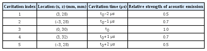
Simulation conditions for the location, relative time, and strength of acoustic emission from five cavitations

Fig. 7.

The time sequence of instantaneous passive cavitation images.

The instantaneous PC image obtained at the occurrence time of cavitation exhibits the best resolution, but to be able to set the time instant, it is necessary to find when cavitation occurs. The instantaneous PC images were computed at intervals of 50 ns from the data of the entire time interval. In the PC image at each time instant, the maximum value of the pixel was found, and the change over time is presented as a graph in Fig. 8A. Five peaks indicating cavitations appear at the same time intervals of 1 μs in Fig. 8B.

Fig. 8.

Five cavitations imaged by tracking temporal variation.

A. Cavitation can be detected using temporal variation of the maximum pixel value of each instantaneous passive cavitation image for the whole time period of radiofrequency data. B. Five cavitation regions (right column) are separated at time instants of cavitation occurrence by placing a circular mask (middle column) around the position of the peak value pixel (left column). It is assumed cavitation 3 occurs at t₀=0 s.

Since the RF data were spread in the time-channel data window, the influence of the side lobe extended to the time range of about ±5 μs, as shown in Fig. 5. The peak value appeared at t=0 s, and the peak values of the other four cavitations with smaller strengths appeared around t=±1 μs and ±2 µs. In Fig. 8, the time at which the peaks appeared was computed using the autofindpeaks function in MATLAB [38]. The occurrence time and relative strength of the five peaks were found to be -2.03 μs (28.6), -1.00 μs (38.5), 0 μs (56.5), 0.98 μs (39.3), and 1.95 μs (27.4) for cavitations 1 to 5, respectively. The region where a cavitation appeared in the instantaneous PC image computed at the time when the peak values appeared in Fig. 8A was separated and shown in Fig. 8B. By creating a circular mask centered on the location of the pixel with cavitation (center column) and multiplying it by the PC image (left column), the cavitation (right column) region from the PC image can be separated. By adjusting the radius of the circular mask, the main lobe region of cavitation can be separated using an image segmentation technique. The separated cavitation images in the right column of Fig. 8B were superimposed to obtain the overall cavitation distribution and relative strength shown in Fig. 9A and B. The high-resolution instantaneous PC image in Fig. 9C and D indicates that the widespread side lobe is essentially removed and that the main lobe region is also reduced compared with the integrated PC image. Fig. 9E shows the integrated PC image obtained by collecting data over the entire time duration. The five cavitations that can be distinguished appear with different signal levels. The spatial resolution of the main lobe representing cavitation is low, and large side lobe levels appear in a wide area.

Fig. 9.

The superposition of five detected cavitations.

The superposition of five detected cavitations produces a highresolution passive cavitation (PC) image in which the locations and relative strengths of five cavitations can be identified: circular masks at detected cavitation positions (A); high-spatial-resolution cavitation image with side lobe masked out, two-dimensional cavitation map of five detected cavitations (B); map of relative strength (C); map of occurrence time (D); and integrated PC image of five cavitations (E).

Discussion

The proposed method constructs an instantaneous PC image with temporal resolution by using the delay and sum focusing method employed in a conventional medical ultrasound imaging system. However, as shown in Fig. 4, a single cavitation shows a large side lobe near the cavitation position for a long time. Therefore, it is necessary to compute the time when cavitation occurs by tracking the temporal change in the cavitation signal strength in instantaneous PC images. Fig. 5 plots a graph of the maximum pixel value in each of the instantaneous PC images. The occurrence time of cavitation was determined by finding the time instant at which the maximum value appeared.

Since high-spatial-resolution instantaneous PC imaging computes only the PC image at the time of cavitation occurrence, there is no accumulation of side lobes, and high-resolution images can be attained. However, as shown in Fig. 5, large side lobes are generated for a long time (a time interval of about 10 µs) before and after cavitation occurrence. Therefore, as shown in Fig. 8, in the case of multiple cavitations, where small cavitations occur in temporal proximity to the large cavitation signal, the main lobe of the small cavitation is swamped in the side lobe of the large cavitation, and thus the peak values of small signals in the graph of the maximum magnitude versus time cannot be detected. Thus, the proposed method can distinguish and separate the individual cavitations only if the cavitation occurrence time instants do not coincide so that the main lobe signal is not masked by each side lobe.

An ultrasound image can be modeled as a convolution of the PSF of a focusing system and the distribution (mainly, position and reflectivity) of scatterers. Accordingly, assuming that a cavitation is a point-like source, the cavitation is manifested as a main lobe of the PSF in an ultrasound image. A bubble generated in water due to the shock wave takes the form of a sphere when photographed [5,39]. However, the cavitations in Figs. 3 and 9 appear to be ellipses with the major axis along the axial direction. Therefore, we can see that the ultrasound PC image does not exactly convey the physical shape of a cavitation. Fig. 9C and D depict a two-dimensional map of the relative strength and occurrence time of each cavitation, respectively.

The conventional cavitation image showed a map of the power by integrating the cavitation signal because the strength of each cavitation could not be determined [14]. Since the proposed method detects the strength of each cavitation, we have used it to express the magnitude of cavitation.

The proposed method is effective in imaging each cavitation event separately when cavitations do not occur simultaneously and the distance between them is not small, as in the case that the frequency of cavitation occurrence is low, which is the case for shock wave therapy. In Fig. 5, the range of time over which the side lobes have an effect amounts to 10 μs. As a result, multiple cavitations that occur in close temporal proximity and whose strength is smaller than side lobe levels are not amenable to detection. Furthermore, when several cavitations appear simultaneously in an instantaneous PC image, only a single maximum brightness is detected in the proposed PC imaging method. Work is in progress to distinguish multiple cavitations that occur simultaneously in instantaneous PC imaging.

Although the effectiveness of treatment in histotripsy increases with increasing cavitation density, it is difficult to distinguish individual cavitations considering the state-of-the-art resolution available in current ultrasound imaging systems. In this case, it is sufficient to show the spatial distribution of cavitation activity. The method proposed herein was developed for the purpose of monitoring cavitation activities in real time under the condition that individual cavitations can be distinguished.

The method proposed in this study is advantageous in that individual cavitations can be identified and that their occurrence time, location, and strength can also be determined by only detecting the main lobe peak with reduced computational complexity. Furthermore, a high-resolution PC image can be obtained by completely removing side lobes, which have plagued the conventional PC imaging methods.

The proposed new PC imaging method can be readily incorporated into a conventional ultrasound diagnostic device, and practically used to monitor the treatment process in the field of therapeutic ultrasound (e.g., extracorporeal shockwave lithotripsy, extracorporeal shockwave therapy, high-intensity focused ultrasound, and histotripsy) where inertial cavitation is an important mechanism of treatment. Further studies are required to confirm the clinical usefulness of the proposed method and to expedite its clinical application.

Notes

Author Contributions

Conceptualization: Jeong MK, Choi MJ, Kwon SJ. Data acquisition: Jeong MK. Data analysis or interpretation: Jeong MK, Choi MJ, Kwon SJ. Drafting of the manuscript: Jeong MK, Choi MJ, Kwon SJ. Critical revision of the manuscript: Jeong MK, Choi MJ, Kwon SJ. Approval of the final version of the manuscript: all authors.

Mok Kun Jeong and Min Joo Choi serve as editors of Ultrasonography, but had no role in the decision to publish this article. All the authors declared no conflicts of interest.

Acknowledgements

This work was supported by research grants from the National Research Foundation of Korea (Grant No. 2017R1A2B3007907) and the Korean Medical Device Development Fund grant funded by the Korean government (the Ministry of Science and ICT, the Ministry of Trade, Industry and Energy, the Ministry of Health and Welfare, and the Ministry of Food and Drug Safety) (1711134987, KMDF_PR_20200901_0010).

References

1. Bailey MR, Khokhlova VA, Sapozhnikov OA, Kargl SG, Crum LA. Physical mechanisms of the therapeutic effect of ultrasound (a review). Acoust Phys 2003;49:369–388.

2. Bailey MR, McAteer JA, Pishchalnikov YA, Hamilton MF, Colonius T. Progress in lithotripsy research. Acoust Today 2006;2:18–29.

3. Cleveland RO, McAteer JA. The physics of shock wave lithotripsy. In : Smith AD, Badlani GH, Bagley DH, Clayman RV, Docimo SG, Jordan GH, et al, eds. Smith’s textbook of endourology 2nd edth ed. London: BC Decker; 2006;:317–332.

4. Leighton TG, Cleveland RO. Lithotripsy. Proc Inst Mech Eng H 2010;224:317–342.

5. Xu Z, Raghavan M, Hall TL, Chang CW, Mycek MA, Fowlkes JB, et al. High speed imaging of bubble clouds generated in pulsed ultrasound cavitational therapy: histotripsy. IEEE Trans Ultrason Ferroelectr Freq Control 2007;54:2091–2101.

6. Xu Z, Raghavan M, Hall TL, Mycek MA, Fowlkes JB. Evolution of bubble clouds induced by pulsed cavitational ultrasound therapy: histotripsy. IEEE Trans Ultrason Ferroelectr Freq Control 2008;55:1122–1132.

7. Mancia L, Rodriguez M, Sukovich J, Xu Z, Johnsen E. Single-bubble dynamics in histotripsy and high-amplitude ultrasound: modeling and validation. Phys Med Biol 2020;65:225014.

8. Dubinsky TJ, Khokhlova TD, Khokhlova V, Schade GR. Histotripsy: the next generation of high-intensity focused ultrasound for focal prostate cancer therapy. J Ultrasound Med 2020;39:1057–1067.

9. Pahk KJ, Dhar DK, Malago M, Saffari N. Ultrasonic histotripsy for tissue therapy. J Phys Conf Ser 2015;581:012001.

10. Xu Z, Hall TL, Vlaisavljevich E, Lee FT Jr. Histotripsy: the first noninvasive, non-ionizing, non-thermal ablation technique based on ultrasound. Int J Hyperthermia 2021;38:561–575.

11. Suarez Escudero D, Goudot G, Vion M, Tanter M, Pernot M. 2D and 3D real-time passive cavitation imaging of pulsed cavitation ultrasound therapy in moving tissues. Phys Med Biol 2018;63:235028.

12. Burgess MT, Apostolakis I, Konofagou EE. Power cavitation-guided blood-brain barrier opening with focused ultrasound and microbubbles. Phys Med Biol 2018;63:065009.

13. Yang Y, Zhang X, Ye D, Laforest R, Williamson J, Liu Y, et al. Cavitation dose painting for focused ultrasound-induced blood-brain barrier disruption. Sci Rep 2019;9:2840.

14. Davies HJ, Morse SV, Copping MJ, Sujarittam K, Bourgin VD, Tang MX, et al. Imaging with therapeutic acoustic wavelets: short pulses enable acoustic localization when time of arrival is combined with delay and sum. IEEE Trans Ultrason Ferroelectr Freq Control 2021;68:178–190.

15. Li T, Khokhlova TD, Sapozhnikov OA, O'Donnell M, Hwang JH. A new active cavitation mapping technique for pulsed HIFU applications: bubble Doppler. IEEE Trans Ultrason Ferroelectr Freq Control 2014;61:1698–1708.

16. Gateau J, Aubry JF, Pernot M, Fink M, Tanter M. Combined passive detection and ultrafast active imaging of cavitation events induced by short pulses of high-intensity ultrasound. IEEE Trans Ultrason Ferroelectr Freq Control 2011;58:517–532.

17. Worthington AE, Sherar MD. Changes in ultrasound properties of porcine kidney tissue during heating. Ultrasound Med Biol 2001;27:673–682.

18. Haworth KJ, Salgaonkar VA, Corregan NM, Holland CK, Mast TD. Using passive cavitation images to classify high-intensity focused ultrasound lesions. Ultrasound Med Biol 2015;41:2420–2434.

19. Salgaonkar VA, Datta S, Holland CK, Mast TD. Passive cavitation imaging with ultrasound arrays. J Acoust Soc Am 2009;126:3071–3083.

20. Jensen CR, Ritchie RW, Gyongy M, Collin JR, Leslie T, Coussios CC. Spatiotemporal monitoring of high-intensity focused ultrasound therapy with passive acoustic mapping. Radiology 2012;262:252–261.

21. Ikeda T, Yoshizawa S, Koizumi N, Mitsuishi M, Matsumoto Y. Focused ultrasound and lithotripsy. Adv Exp Med Biol 2016;880:113–129.

22. Macoskey JJ, Choi SW, Hall TL, Vlaisavljevich E, Lundt JE, Lee FT, et al. Using the cavitation collapse time to indicate the extent of histotripsy-induced tissue fractionation. Phys Med Biol 2018;63:055013.

23. Ebbini ES, ter Haar G. Ultrasound-guided therapeutic focused ultrasound: current status and future directions. Int J Hyperthermia 2015;31:77–89.

24. Coleman AJ, Choi MJ, Saunders JE, Leighton TG. Acoustic emission and sonoluminescence due to cavitation at the beam focus of an electrohydraulic shock wave lithotripter. Ultrasound Med Biol 1992;18:267–281.

25. Bailey MR, Pishchalnikov YA, Sapozhnikov OA, Cleveland RO, McAteer JA, Miller NA, et al. Cavitation detection during shockwave lithotripsy. Ultrasound Med Biol 2005;31:1245–1256.

26. Khokhlova VA, Fowlkes JB, Roberts WW, Schade GR, Xu Z, Khokhlova TD, et al. Histotripsy methods in mechanical disintegration of tissue: towards clinical applications. Int J Hyperthermia 2015;31:145–162.

27. Jeong MK, Kwon SJ. Side lobe free medical ultrasonic imaging with application to assessing side lobe suppression filter. Biomed Eng Lett 2018;8:355–364.

28. Jeong MK, Kwon SJ. A new method for assessing the performance of signal processing filters in suppressing the side lobe level. Ultrasonography 2021;40:289–300.

29. Jones RM, McMahon D, Hynynen K. Ultrafast three-dimensional microbubble imaging in vivo predicts tissue damage volume distributions during nonthermal brain ablation. Theranostics 2020;10:7211–7230.

30. Coviello C, Kozick R, Choi J, Gyongy M, Jensen C, Smith PP, et al. Passive acoustic mapping utilizing optimal beamforming in ultrasound therapy monitoring. J Acoust Soc Am 2015;137:2573–2585.

31. Lyka E, Coviello CM, Paverd C, Gray MD, Coussios CC. Passive acoustic mapping using data-adaptive beamforming based on higher order statistics. IEEE Trans Med Imaging 2018;37:2582–2592.

32. Thomenius KE. Evolution of ultrasound beamformers. In : In: 1996 IEEE International Ultrasonics Symposium; 1996 Nov 3-6; San Antonio, TX, USA. Piscataway, NJ: Institute of Electrical and Electronics Engineers; 1996. 1615–1618.

33. Norton SJ, Won IJ. Time exposure acoustics. IEEE Trans Geosci Remote Sens 2000;38:1337–1343.

34. Kamimura HAS, Wu SY, Grondin J, Ji R, Aurup C, Zheng W, et al. Real-time passive acoustic mapping using sparse matrix multiplication. IEEE Trans Ultrason Ferroelectr Freq Control 2021;68:164–177.

35. McLaughlan J, Rivens I, Leighton T, ter Haar G. A study of bubble activity generated in ex vivo tissue by high intensity focused ultrasound. Ultrasound Med Biol 2010;36:1327–1344.

36. Li M, Gu J, Vu T, Sankin G, Zhong P, Yao J, et al. Time-resolved passive cavitation mapping using the transient angular spectrum approach. IEEE Trans Ultrason Ferroelectr Freq Control 2021;68:2361–2369.

37. Ustuner KF, Holley GL. Ultrasound imaging system performance assessment. In : In: 45th AAPM Annual Meeting; 2003 Aug 10-14; San Diego, CA, USA. Alexandria, VA: American Association of Physicists in Medicine; 2003. 10–14.

38. O’Haver TC. A pragmatic introduction to signal processing with applications in scientific measurement [Internet]. The Author 2008. [cited 2021 Jul 21]. Available from: https://terpconnect.umd.edu/~toh/spectrum/PeakFindingandMeasurement.htm.

39. Pahk KJ, de Andrade MO, Gelat P, Kim H, Saffari N. Mechanical damage induced by the appearance of rectified bubble growth in a viscoelastic medium during boiling histotripsy exposure. Ultrason Sonochem 2019;53:164–177.

Article information Continued

This is an Open Access article distributed under the terms of the Creative Commons Attribution Non-Commercial License (http://creativecommons.org/licenses/by-nc/4.0/) which permits unrestricted noncommercial use, distribution, and reproduction in any medium, provided the original work is properly cited.

Notes

Key point

Conventional integrated passive cavitation imaging constructs an image by obtaining the focused signals at all times, but does not provide information on when cavitation occurs. To solve this problem, we apply instantaneous passive cavitation imaging to passively received radiofrequency data in the beamforming process, detect the position and time of each bubble burst, and suppress side lobes. The proposed method can be readily integrated into a diagnostic ultrasound scanner to monitor the treatment process of shock wave therapy and histotripsy where cavitation is an important mechanism.

Cavitation index	Location (x, z) (mm, mm)	Cavitation time (μs)	Relative strength of acoustic emission
1	(3, 28)	t₀-2 μs	0.5
2	(-3, 28)	t₀-1 μs	0.7
3	(0, 30)	t₀	1.0
4	(3, 32)	t₀+1 μs	0.7
5	(-3, 28)	t₀+2 μs	0.5